Ok, so the title might just have outed my love for all things Lebowski, but hopefully I will be able to make a link, irregardless of how tenuous it might be, between tumbleweeds and and the subject of this post, drifters.

First things first, we have to remind ourselves what is a drifter, and how does it differ from a float.  First, drifters float and floats sink, yes, this is correct, floats sink, drifters don’t.  Drifters, or more precisely, passive Lagrangian drifters (PLD), are the kind we deploy during NAAMES in the North Atlantic. These are basically big bobbers which are “anchored” to the surface ocean by an amalgamation of fabric (at times brightly colored in pink camouflage), metal and plastic that is called a “holy sock drogue.”  Maybe a picture will help, with the visual aid of me in the holy sock drogue.

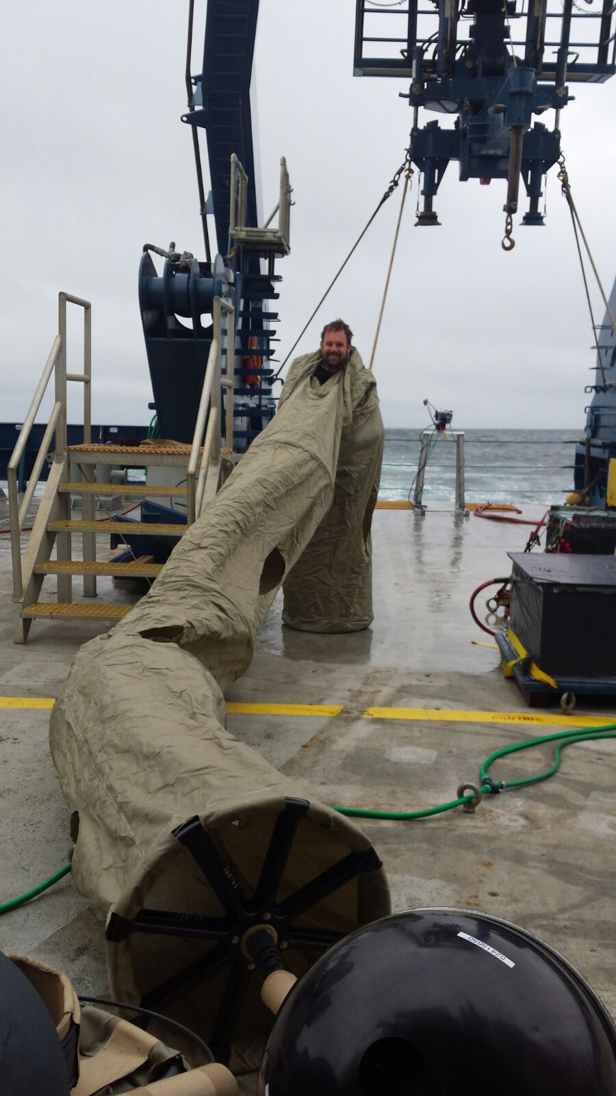
This is a Pete inside a drifter.  The “sock” is about 10 m long and helps to anchor the drifter into the ocean surface currents.

Ok, so what do these drifters do?  Think of them as a breadcrumb trail that we drop and leave behind the boat.  We drive this big ship through the ocean and choose what might seem to be random spots to stop and sample.  The truth is these spots are not random. They are the result of the integration of lots of satellite observations, and at times, data we get from the floats (that sink), all which help us decide where we want to sample.  Once we arrive “on station”, we drop three of these drifters.  I’ll go into details as to why we drop three of them later, but for now, think of this as the breadcrumbs we drop to mark the water mass where we have sampled.  Since the ocean is always moving, the drifter moves along with the surface layer of the ocean and allow us to follow them in time in order to stay with the same “water mass” that we initially sampled.  During the NAAMES project, we also have a big airplane that samples not only the air, but also shoots a laser into the ocean to measure phytoplankton from the surface to about 50 m.  Using the drifters, the plane can sample the same water mass that we sampled with the ship a few days prior.

So why drop three of the $3,000 drifters at once you may ask?  Well, these drifters allow us to measure something that is actually really hard to measure in the ocean, that is diffusion.  Diffusion is basically how fast do things spread apart, and how does this “rate of spreading” change based on where we dropped the drifters.  Together with other members of the (Sub)mesoscale Group, we will use the rate at which these drifters spread in time to estimate how mesoscale eddies influence the diffusion of the oceans surface waters.  To do this, we get hourly updates on the positions of all the drifter and compute the evolution of the area between the three drifters over time.  All this fun stuff won’t get analyzed for some time as we need to allow enough time for all the drifters to spread apart.

In addition to dumping drifters on station, Ali and I have designed

Deploying drifters is fun!  The (Sub)mesoscale Group is all about having fun while doing cutting-edge science.

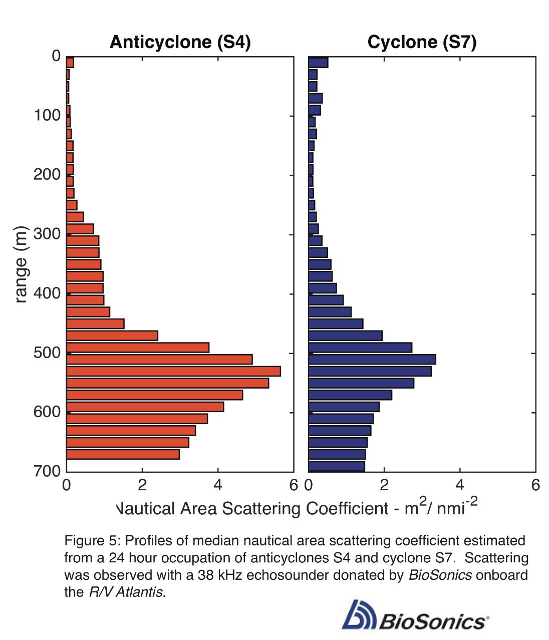
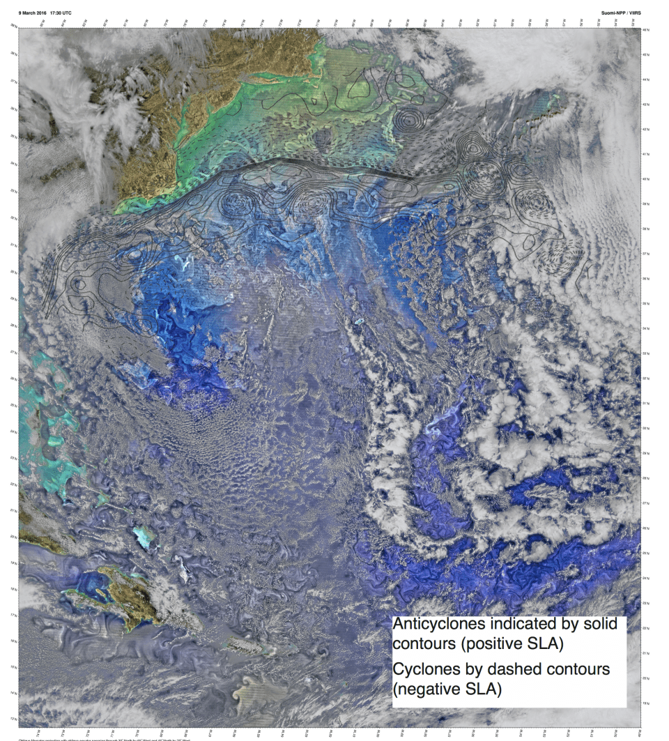
a few diffusion experiments.  We deployed (fancy word for dumped) triplicate drifters: outside of eddies, on the edge of eddies, at the point in the eddy where currents are at a maximum, and at the eddy center.  This will allow us to compute how eddies influence diffusion and compare how the impact of these eddy varies between cyclones and anticyclones (i.e., the cold and warm core eddies).

But enough with all this science, we also have fun.  It’s cool to deploy drifters as it’s a neat feeling to put out an instrument that talks with a satellite every hour for the next few years!  For example, we deployed drifters in the middle of a warm core ring, which is a really big and strong eddy that is shed from the Gulf Stream (see some details about our warm core ring project here).  One of these drifter stayed in the ring for a few days making larger loops around the eddy.  In addition, superimposed on the big loops, were small little loops that are the result of what we call inertial motions.  Basically, because the Earth rotates, surface water in the ocean oscillates in little circles all day, every day.  After a few days, the drifter was spit out of the eddy and started heading clear across the Gulf Steam.  The resulting drifter track was a very pretty pattern reminiscent of a rose.

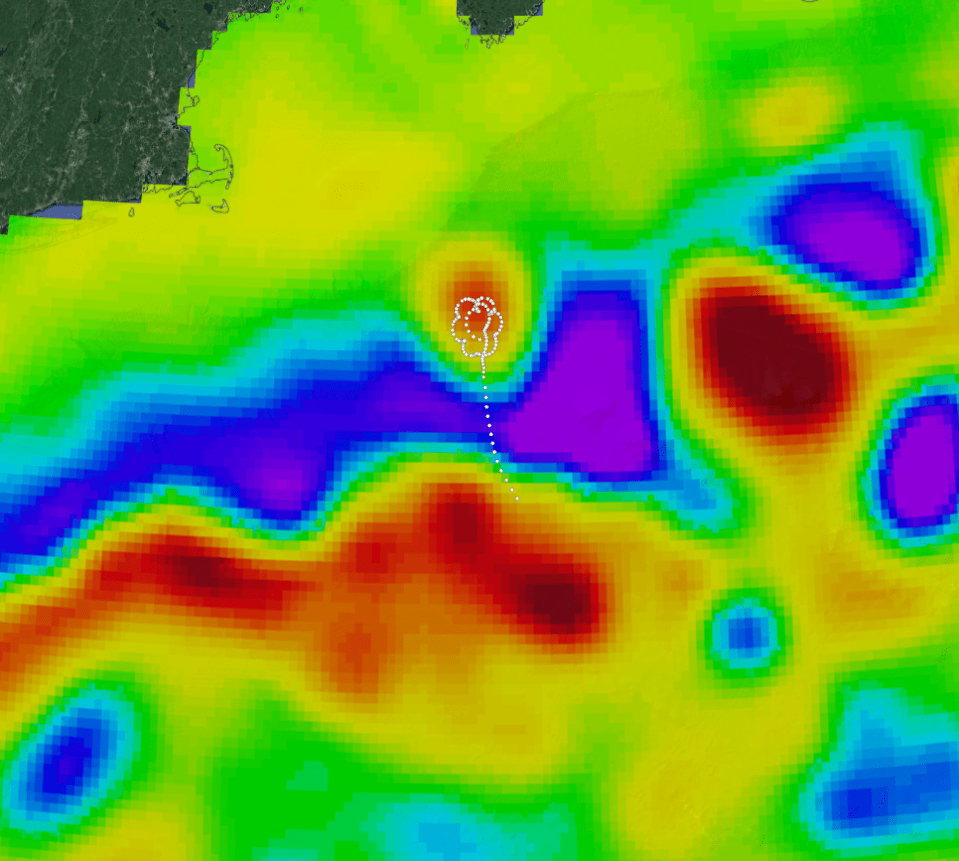
A drifter traces a rose in a warm core ring.

To wrap up, drifters drift, just as the proverbial tumbleweed, allowing us to follow a mass of water to sample with the ship and plane.  Sometimes the patterns made by the drifters are really pretty, like our rose.

Post by Alice Della Penna

When we think about the ocean, our first reflex might be to imagine the blue of a paradise tropical island or massive waves hitting remote cliffs on a stormy night. The most adventurous may think about submarines exploring the deep ocean and rovers sampling underwater volcanoes. There is something extremely fascinating that sits right “in the middle” of these two worlds and that is largely unexplored. The so-called mesopelagic extends between depths of 200 and 1,000 m below the ocean surface, between the daily lit epipelagic, where famous sea-life such as phytoplankton and dolphins live, and the dark bathypelagic, where no sun light penetrates.

The mesopelagic is also called the “ocean twilight zone” because it is located between the epipelagic ocean, closer to the ocean surface and the deep sea, that is never reached by the light. (Credit: Wikipedia/Creative Common)

Being far from the ocean surface, where photosynthesis empowers epipelagic ecosystems, one would expect the mesopelagic to be relatively empty. Instead, sonar operators and scientists found out that the mesopelagic hosts an extremely rich ecosystem, so dense in life that layers of fish and zooplankton [planktonic animals that include small crustaceans (including krill), jelly-like organisms, arrow worms that feed mainly on phytoplankton] can foul sonars creating the illusion of a false bottom! Recent studies estimate that the mesopelagic is likely to host about 10^9 tons (yes, it’s 10 with other 8 zeros behind it) of fishes, without counting crustaceans, squids and other animals that inhabit the so-called deep scattering layer.

To make things even more mysterious, part of the organisms that create the deep scattering layer migrate every sunset from the deep sea to the epipelagic, where they are thought to feed on phytoplankton and are eaten by a range of ocean predators. (Some predators actually feed on them also during the day, by performing extremely deep dives in the mesopelagic). Then, when the sun rises again, they swim back to the deep ocean. This phenomenon is called diel vertical migration and is  the largest animal migrations on Earth, and it happens twice a day! Even if it involves “only” displacements of hundreds of meters, it is experienced by small (of a thumb-size and less) animals. I will never complain about my commute again.

Very little is known about this “world” and its interaction with the ocean epipelagic. What are mesopelagic organisms eating exactly? And how much? What do they do during the day? What triggers their migrations (likely light, as in sun-up, sun-down)? How does their movement affect the cycles of different elements (especially carbon, the building blocks of life)? How are they affected by the variability in the ocean conditions at the surface? Are they distributed in the same way in different regions in the ocean? There is a lot of work to do!

During the NAAMES research voyage we are trying to learn something about the mesopelagic in the North Atlantic in different ways. Every time the ship slows down to ~ 4 knots, we put in the water our acoustic system: the echosounder. The idea is similar to the one behind a fancy fish finder, a sonar or the way bats find their dinner: our instrument sends sound towards the deep ocean and some of the signal is reflected by surfaces with different density (for example fish bladders). By measuring the time between when the sound is sent and when it is received back and the intensity of the reflected signal, we can estimate how much “stuff” is at which depth. We do that at different frequencies so that we can describe the distribution of organisms of different sizes, but unfortunately we cannot visually “see” what’s there.

An example of the output from the echosounder from NAAMES 2 (May 2016). The x-axis shows time (in particular, the time of the day) and the y-axis shows depth. Different colors refer to the intensity of the reflected signal from different depths (i.e. red and yellow mean that there is a lot of “backscatterers”/ stuff that reflects sound, white that there is very little / nothing and blue and green represent intermediate values. This plot shows the output of the echosounder for 2 days and it’s possible to see the vertical migration of some mesopelagic organisms at sunset and sunrise.

Another tool we use to explore the mesopelagic is a net. At each station, we have a look at our echosounder and we decide at which depth we will tow our net. SSSG and crew members team up with us to put our big net at the right depth and drive the winch to tow it for a time between 40 minutes and 2 hours. When the net is brought back up to the surface it is hard not to be excited: the net is coming from the mesopelagic and we could find anything in there! After taking out our “catch” and rinsing the gear (that tends to be vaguely stinky for a while), it’s time to look at what we got: according to the location and the “layer” we targeted, so far we got a good selection of shrimp-like crustaceans, jelly-like zooplankton and a good collection of mesopelagic fish.

Examples of mesopelagic fish and zooplankton from our net tow.
(1- Hatchetfish, 2- Myctophid, 3- Bristlemouth, 4- A crustacean).
Photos by Stuart Halewood

It will be definitely fun and interesting to compare the results from our net-tow from different stations, with patterns in the echosounder and with the results of the “imaging team” that are taking snapshots of zooplankton at different depths during the water sampling sessions.

We’re getting good at this whole (sub)mesoscale survey thing.  With an enthusiastic crew we left Newport just after 6am heading 25 miles offshore into “deep water.”  Overall, the day was uneventful, thus it was perfect.  All instruments, crew, and boat returned to dock in working condition.

We conducted two 10+ km survey with multiple CTDs, backscattering, two-freq echosounder, and a two-freq ADCP.  All in all, we are starting to accumulate a good deal of great data using the small boat.

We’re proud, we have developed a way to survey submesoscale features in the open ocean using a “small” boat with minimal cost.  Our first survey was a success.  Energized by this, we leave the dock at sunrise with calm seas. We clear any tidal debris in the first 15 miles from port.  We are moving comfortably at 22 knots when I feel a small thump at my feet.  Engine immediately reeves and we loose speed.  

Kristina sees a oceanic sunfish (Mola Mola) flopping at the surface behind the boat, it’s a big one, a real big one.  After I mount the small outboard, we approach the Mola to take a picture right as it disappears into the deep blue.

I assume my position on the till for the next 5 hours as Kristina sends hourly updates to the Coast Guard.

After a long day going really slow, we pull the boat to find that striking the Mola removed the entire lower unit, we’re happy we did not take on water.

Lesson learned, you can’t always see a Mola to avoid it, therefore, hope for the best and make sure you do all you can to stay lucky.

Expanding on our ability to make cutting-edge measurements from small boats in the open ocean, we joined Capt. Perry Chrisler onboard the C’est si Bon to survey from Cabo San Luca, Mexico to San Diego, CA; the length of Baja.

Unfortunately, our primary instrument flooded on day 1.  We resorted to “old school” ocean observations measuring currents by differences in speed over ground versus speed through the water and making detailed notes on all that we saw.  We ended up proving that we are able to conduct (sub)mesoscale underway CTD survey from sailing ships using very little fuel and power and collect observations along fronts using binoculars and a note book.  As a bonus, we feasted on raw yellowfin tuna for 10 days.

In addition, both Cam and I learned a lot about sailing, and bashing, as they say. Unfortunately, after a long winter in the North, the two weeks we had in Baja were colder than either in Seattle or Boston, but hey, it wasn’t a vacation.

We will return, with more instruments, and always a spare of everything we put in the water.

We collected a good amount of interesting data before the storm.  Come 2am, the storm was upon us and the winds swiftly picked up to 50 knots.  I thought my transducer pole would be safe if in the down position with the guide rope attached.  As it turns out, nothing was safe.

3am: Enjoying watching 30′ waves crush the stern of the ship.

4am: I realized that the pole might not fair well and decided to disconnect the echosounder.

5am: Capt. informs me that he doesn’t think the pole will make it through the storm (this is when the video was taken).  Front guide rope snaps.

6am: The pole breaks loose and is bashing the side of the ship as it hangs on with a single kevlar rope, captain send the crew to cut it loose.  I shed a tear and then start to plan on how to replace all the instruments.

Lesson learned, now I carry insurance.

We returned to the North Atlantic in May to continue trying to understand why white sharks might be foraging in anticyclonic eddies.  As sometimes happens, we were surprised to learn that in anticyclonic eddies (ocean desert) the amount of stuff (biomass) in mesopelagic ecosystems (those at depths of 200 – 1,000 m) appears to have an inverse relationship with phytoplankton biomass at the surface.

In preparation for our May expedition to characterize the variability of phytoplankton, zooplankton, and mesopelagic fish and squid in the North Atlantic, we wanted to compare the location of mesoscale eddies observed in maps of sea level anomalies with a stunning image of ocean color (phytoplankton) generated by NASA.

There are a number of interesting features that can be seen both in the altimeter data (contours) and ocean color, including cold-core (cyclonic) eddies south of the Gulf Stream and warm-core (anticyclonic) eddies north of the Gulf Stream.

This comparison of the high-resolution ocean color image (pixels are between 500m and 1km in size) with contours of the AVISO sea level product (with pixels of ~25 km) highlights just how much of the variability in marine ecosystems occurs at scales not resolved by the current generation of satellite altimeters [the submesoscale, O(1-10km)].  Our ability to observed smaller eddies and fronts will be greatly improved with the advent of swath-altmetry (SWOT, launch date around 2020-ish).  At these smaller scales, however, the assumption we use to derive currents from sea level will have to be reconsidered if we are to investigated the dynamics of physical/biological interaction at the submesoscale.

If there is one instrument that can be considered to be the core of sea-going oceanographic research, it’s the CTD package.  CTD stands for Conductivity, Temperature and Depth.  It’s deployed on a long wire from a winch into the depths of the ocean.  The measurements of temperature, salinity (estimated from conductivity) and depth allow us to study the stratification, or layering, of the ocean.  From this we can derive the currents, estimate mixing, and define how close to the surface the plankton are likely to be confined.

But our CTD, or “package” is special.  In addition to the core measurements, we are measuring optical properties of plankton to estimate their biomass and how happy they are.  We also have a little robot that take pictures of all the little beasties that fly by as the “package” goes down to 1,500 m, and then back to the surface.

Deploying the package is quite an ordeal.  The video below shows the process, sped up by 2000%.  Depending on how deep we are doing the cast, or deployment, the whole process takes from 1-3 hours and involves a total of 6 people directly, plus the crew on the bridge who make sure we are always facing into the waves and not in danger.  A crewmember mans the winch, a technician on deck orchestrates the whole ordeal, and four scientists tend the lines and trip the bottles from the computer lab.

CTD_small from Peter Gaube on Vimeo.

Oh yeah, the bottle, argh, those bottles.  In total, there are 24 bottles on the CTD that collectively are called the “rosette.”  These bottles are held open until an electrical signal is sent down the cable to the CTD telling them to snap shut, trapping 10-liters of water in each bottle.  The water is brought to the surface and quickly sampled by a swarm of scientists who analyze the samples for a multitude of measurements, including the rate at which viruses attack plankton, how many plankton there are, how fast they are growing, how green they are, and who is around eating them and at what rate.

Overall, on this field program, and most oceanographic cruises, the backbone of our sampling comes from the CTD package.  I’m just the lucky guy who gets to send it overboard and make sure it comes back on deck safely and full of water.